Protocol

This protocol takes users all the way from constructing a seed dataset through reconstructing ancestors.

Steps done by topiary

The steps covered in this protocol are:

1. Create a seed dataset

2. Generate a multiple sequence alignment from the seed dataset

3. Visually inspect and (possibly) edit the alignment

4. Infer evolutionary trees and ancestors

5. Determine the branch supports on the reconciled tree

6. Interpret outputs and select ancestors

1. Create a seed dataset

The most important task in an ASR study is defining the problem. What ancestors do you want to reconstruct? What modern proteins are best characterized and most relevant to interpreting the results with ancestors? This requires expert knowledge of the proteins under study–it’s not something that can be automated.

The tree for a hypothetical protein family shows how one might approach the problem. Paralog A has some activity (denoted with a star); paralog B does not. If we are interested in the evolution of the star activity, we would likely reconstruct ancA and ancAB (arrows). We expect ancA was active because all of its descendants are active; we expect ancAB was inactive because only the A paralogs–not the B paralogs or fish proteins–are active. Reconstructing ancA and ancAB would thus isolate the key sequence differences that conferred activity.

Two pieces of information specify the scope of the ASR study and thus what ancestors can be reconstructed:

1. What homologs are of interest?

2. What homologs exist in what organisms?

We can think of the answers to these questions graphically. The image below shows the information from above in a different format. The protein family is shown left to right (proteins A-D); the species tree is shown from top to bottom (humans through lampreys). The blue checks and orange exs indicate whether the organism has the protein. To reconstruct ancA and ancAB, we need to know we want to study proteins A and B (paralogs of interest) and we need to know that bony vertebrates, but not other animals, have the A and B proteins (taxonomic scope). The gray box indicates the proteins we need to include in our ASR study to reconstruct ancA and ancAB.

In a topiary calculation, we specify that these are the proteins of interest using a seed dataset. In graphical terms, this means finding sequences representing all paralogs (across horizontal) taken from the full taxonomic scope (the top and bottom of the gray box).

Note

Because the bacterial species tree is poorly defined, topiary will automatically use a taxonomic scope including all bacteria for datasets containing only bacterial proteins.

Prepare a seed dataset as a spreadsheet

A seed dataset defines the paralogs of interest and taxonomic scope for a reconstruction. It has four columns: name (e.g. the paralog), aliases, species, and sequence. Topiary uses this dataset as a starting point for BLAST searches to construct a dataset and generate an alignment for the reconstruction study. An example for the two immune proteins, LY86 and LY96, is shown below. The full spreadsheet can be downloaded here.

name	aliases	species	sequence
LY96	ESOP1;Myeloid Differentiation Protein-2;MD-2;lymphocyte antigen 96;LY-96	Homo sapiens	MLPFLFF…
LY96	ESOP1;Myeloid Differentiation Protein-2;MD-2;lymphocyte antigen 96;LY-96	Danio rerio	MALWCPS…
LY86	Lymphocyte Antigen 86;LY86;Myeloid Differentiation Protein-1;MD-1;RP105-associated 3;MMD-1	Homo sapiens	MKGFTAT…
LY86	Lymphocyte Antigen 86;LY86;Myeloid Differentiation Protein-1;MD-1;RP105-associated 3;MMD-1	Danio rerio	MKTYFNM…

Determine what sequences to include

1. Choose the paralogs of interest for your ASR calculation. As described above, the choice of paralogs determines what evolutionary transitions you will reconstruct. In our experience, you’ll want to select ~1-5 paralogs in your seed dataset. As you add more paralogs, you need more sequences to resolve the evolutionary tree, making the calculation progressively slower. In the example seed dataset, we selected two paralogs, LY86 and LY96.

2. Determine the taxonomic distribution of the protein family. In the graphic above, this means identifying the vertical boundaries of the gray box: which creatures have these proteins? This information is often available through literature searches. The goal is to to identify the most evolutionarily distant groups of organisms that the proteins of interest. For more details on how to determine which organisms have your protein, see this page.

3. Choose two or three species with well-annotated genomes that span the taxonomic distribution of your proteins of interest. In the graphic above, this means selecting species from the top and bottom of the gray box. The human and zebrafish proteins would be a good choice, as they have well-annotated genomes and span the diversity of organisms with the proteins of interest. (Contrast this to selecting humans and chickens, which would only include amniote proteins). The NCBI BLAST “Taxonomy” report from the exploratory BLAST page can be helpful in this regard: select organisms that differ at the highest level of the reported hierarchy.

Construct the seed spreadsheet

The seed dataset is a spreadsheet that can be prepared in a spreadsheet program (Excel or LibreOffice), a text editor, or programmatically via pandas. For technical details on the format of this dataframe, see the documentation.

1. Download sequences for each paralog from each species and put it into the table. Our usual source for these seed sequences is uniprot. Generally, you’ll want the canonical sequence rather than an isoform. These sequences can come from anywhere; they do not even have to be from a database.

2. Compile a list of aliases for each paralog. Annoyingly, the same protein can have different names across different databases/species. By using a human-curated list of aliases, topiary is more effective at identifying sequences that really correspond to the paralogs of interest. When creating this list:

   • separate different aliases with “;”

   • aliases are case-insensitive (i.e. MD2, md2, and Md2 are equivalent)

   • topiary automatically tries different separators. For example, for MD2 topiary will look for MD2, MD 2, MD-2, MD_2, and MD.2. It inserts separators between letters and numbers or any time there is a space/separator in the alias.

   • make sure to include both the abbreviated and full-length versions of each alias (i.e. MD2 and myeloid differentiation protein 2).

   To find aliases, you can check out the “Also known as” field for the gene of interest on NCBI, the “Protein names” section of the protein’s UniProt entry, a “genecards” entry (for proteins found in humans), and/or primary literature.

3. You can put other information about the sequences (accession, citations, etc.) as their own columns in the table. Topiary will ignore, but keep, those columns.

4. If you would like to make sure to include specific sequences in the analysis, you can also add them to the seed dataset. (For example, you might want to make sure an experimentally characterized protein from a specific organism is in the final tree). To do so, add the the sequence to the dataset like any other, then add a fifth column: key_species. Each sequence in the spreadsheet should either have True or False in this column. Those with True will be used as part of the seed dataset; those with False will not be used as seeds, but will be kept in all downstream steps in the analysis. In the following table, we added the mouse sequences to the dataframe as sequences that will be in the final tree but will not be used as seeds for BLAST etc.

   name	aliases	species	sequence	key_species
   LY96	ESOP1;Myeloid Diff…	Homo sapiens	MLPFLFF…	True
   LY96	ESOP1;Myeloid Diff…	Danio rerio	MALWCPS…	True
   LY86	Lymphocyte Antigen…	Homo sapiens	MKGFTAT…	True
   LY86	Lymphocyte Antigen…	Danio rerio	MKTYFNM…	True
   LY86	Lymphocyte Antigen…	Mus musculus	MKTFFNM…	False
   LY96	ESOP1;Myeloid Diff…	Mus musculus	MLSFVYF…	False

2. Generate a multiple sequence alignment from the seed dataset

This step uses the seed sequences as BLAST queries to identify homologs, performs reciprocal BLAST to call the the orthology of the hits, lowers dataset redundancy in an intelligent fashion, and generates a sequence alignment. The steps, as well as output files, are described in detail on the pipelines page.

To run this step, use the following command, replacing seed-dataframe_example.csv with the name of your seed file.

topiary-seed-to-alignment seed-dataframe_example.csv --out_dir seed_to_ali

Note

This can also be run in a Jupyter notebook. For an example, see here. To run this notebook interactively in Google Colab, click the button below.

Output

This will create a directory named seed_to_ali that has a set of csv files that sequentially capture each step in the topiary pipeline, as well as intermediate files used in the calculation. When topiary removes a sequence from consideration, it sets the spreadsheet column keep to False, so you can track how the dataset changes over steps by looking at these spreadsheets.

Tip

If you want to override topiary’s decision to remove a sequence, you can manually set the keep and always_keep columns to True in one of the intermediate spreadsheets. Delete the subsequent spreadsheets and then re-run the pipeline with the --restart argument described above. That sequence will now be kept regardless of quality score or redundancy.

The outputs used for the next step are seed_to_ali/05_clean-aligned-dataframe.csv and seed_to_ali/06_alignment.fasta. The final csv file is a topiary dataframe that has only the final sequences and information about them. The fasta file holds the final alignment.

Note

Generally, this script should take less than an hour. The time required for the initial NCBI BLAST step depends on server capacity and may take a while. Unfortunately, this is outside of topiary’s control. If this step is too slow or crashes, you can load in sequences from saved BLAST XML files using the –blast_xml argument to topiary-seed-to-alignment.

Options

There are many options available for this function. These can be accessed by:

topiary-seed-to-alignment --help

Some of the more common options users might wish to change are listed below.

Controlling alignment size

The --seqs_per_column and --max_seq_number arguments control how many sequences topiary will attempt to place in the final alignment. By default, topiary will attempt to have one sequence per amino acid in the average seed sequence (--seqs_per_column 1). For example, if your average seed is 200 amino acids long, it will aim for 200 sequences in the alignment. This can be changed by changing the value of --seqs_per_column. The maximum alignment size is set by --max_seq_number. Note that these values are approximate; the final alignment may be slightly larger or smaller.

Choosing different BLAST inputs

You can select different BLAST inputs via the --blast_xml, --ncbi_blast_db, and --local_blast_db options. Any combination of these options may be specified at the same time, allowing a single command to BLAST against an NCBI database, BLAST against a local BLAST database, and load results from a collection of previously saved BLAST XML files. The --blast_xml option is particularly useful, as you can save NCBI BLAST results from the web interface (for example) and read those files in directly.

Restarting

You can restart a command from an existing directory using a command like the following:

topiary-seed-to-alignment seed-dataframe_example.csv --out_dir seed_to_ali --restart

This will find the last completed step in the pipeline and will restart the pipeline from there.

3. Visually inspect and (possibly) edit the alignment

Before reconstructing a phylogenetic tree and ancestors, we recommend inspecting and possibly editing the alignment. We recommend using Aliview for this purpose.

Danger

Topiary will give you the best-aligning set of sequences given the BLAST results, but it does not assess absolute alignment quality. If the sequences are so divergent that they cannot be aligned reliably, the downstream ASR steps will not be successful. Things to look for are protein regions with variable lengths and sequences (such as loops and extensions) as well as highly divergent sequences where there is no clear shared set of amino acids with other sequences. Ancestral sequences for such regions will be impossible to reconstruct with confidence.

There are differing views on whether or not to manually edit an alignment. Manual edits are subjective, but there are also “obvious” instances where automatic alignment software does poorly. We usually edit our alignments using the following protocol.

If you modify your alignment manually, it should be included in any publication so others can reproduce/evaluate your work. We recommend including the final topiary .csv file as a supplemental file with your manuscript, as this has all sequence accessions and the final alignment in a single table.

Danger

When editing the alignment, do not change the names of the sequences as this is how topiary maps the alignment back into the dataframe. Likewise, do not add sequences to the alignment. (To add sequences, you should add them to the dataframe itself before writing out the alignment.)

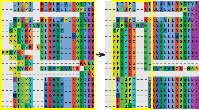
Trim variable-length N- and C-terminal regions from the alignment. A huge number of sparse and variable columns will slow evolutionary analyses and will generally not provide enough signal to be reconstructed with confidence.

Delete sequences with long, unique insertions or deletions (indels). Indels can lead to alignment ambiguity around flanking regions. Further, they provide no information for most ancestors, most of whom do not have the indel, while increasing the computational cost of the phylogenetic analysis. Note, do not make internal edits to sequences (say, by deleting a long lineage-specific insertion) as this becomes difficult to track or justify upon future realignment steps.

Delete lineage-specific duplicates. Select the sequence with the greatest sequence coverage. The pipeline generally does a good job of deleting sequences in this class; however, if such sequences slip through, delete them from the alignment.

Globally realign the sequences. Because trying to align long and variable sequences like those we deleted above can affect the alignment of other sequences, we generally use Muscle5 to re-align the entire dataset after we remove problematic sequences and columns. Alignment can be done directly within AliView. We often iterate through the steps above and full realignment several times.

Carefully inspect the alignment and correct “obvious” local misalignments. Shift characters, without deleting characters, to correct identical or nearly identical regions that are misaligned. This can occur at the edges of insertions and deletions.

Once you are satisfied with the alignment, save it out as a .fasta file from your alignment editor.

Load the final alignment into the dataframe

Once you have edited the alignment, load the new alignment back into a new, final topiary dataframe.

topiary-fasta-into-dataframe 05_clean-aligned-dataframe.csv edited_alignment.fasta final_dataframe.csv

In this command, edited_alignment.fasta should be the name of the fasta file you saved out above. final_dataframe.csv is the name of the final csv file. The file final_dataframe.csv can then be used for all subsequent reconstruction steps.

4. Infer evolutionary trees and ancestors

This step will do five tasks:

• Infer the maximum likelihood model of sequence evolution

• Infer a maximum likelihood gene tree

• Infer ancestors on the maximum likelihood gene tree

• Generate bootstrap replicates for the maximum likelihood gene tree

• Reconcile the gene and species trees (for non-microbial proteins)

The input for this calculation is the .csv file from the last step. A small example input file can be found here. This dataset will take about an hour to run on a laptop.

We highly recommend running the this analysis on a computing cluster. To prepare the computing environment, please install topiary on the cluster. The following instructions assume you installed topiary in a conda environment named topiary.

Note

You can run this as a Jupyter notebook instead of using the command line. For an example, see this notebook. To run this notebook interactively (for a toy dataset) on Google Colab, click the button below.

Copy the final dataframe up to the cluster.

scp final_dataframe.csv username@my.cluster.edu:

Running topiary on a cluster will require a run file that specifies the resources available for the calculation. The following is an example SLURM script for our local cluster. (Check with your cluster administrator for the relevant format.)

#!/bin/bash -l
#SBATCH --account=harmslab
#SBATCH --job-name=topiary
#SBATCH --output=hostname.out
#SBATCH --error=hostname.err
#SBATCH --partition=long
#SBATCH --time=07-00:00:00
#SBATCH --nodes=1
#SBATCH --ntasks-per-node=28
#SBATCH --cpus-per-task=1

# Activate the topiary conda environment
conda activate topiary

topiary-alignment-to-ancestors final_dataframe.csv --out_dir ali_to_anc --num_threads 28

The key aspects to note in this file are:

• The number of threads should match between the topiary call (--num_thread 28) and the cluster resource allocation (#SBATCH --ntasks-per-node=28).

• This script should be run on a single physical processor (#SBATCH --nodes=1). This is because the conda version of RAxML-NG is not compiled to parallelize across multiple processors.

• We’ve found that this step usually takes a few days for an alignment with ~500 sequences and ~1000 columns. We conservatively allocated a week (#SBATCH --time=07-00:00:00).

• If you installed topiary using conda (as we recommend), you need to make sure that the conda environment is active (conda activate topiary).

You start the topiary run using something like the following command. This is for SLURM on our cluster; check with your administrator for the appropriate command on your system.

sbatch launcher.srun

Output

The output for this call is a directory (ali_to_anc from command above). The primary output is ali_to_anc/results/index.html. This file summarizes the results of the calculation. The results directory is a self-contained unit that can be shared and opened by anyone, even if they do not have topiary installed. The ali_to_anc directory will also have directories for each step in the pipeline. For details about these directories and the functions called in the pipeline, see the pipelines page.

Options

To see the options available for this function, type:

topiary-seed-to-alignment --help

Some of the more important options are:

• --restart. This allows you to restart a partially completed job.

• --force_reconcile and --force_no_reconcile. This will force the gene tree and species trees to be reconciled, overriding the default. (The default is to not reconcile for microbial datasets and to reconcile for non-microbial datasets).

• --horizontal_transfer. This selects whether reconciliation will allow horizontal transfer of genes. By default, this is not allowed. This is only meaningful if the gene and species trees are being reconciled.

5. Determine the branch supports on the reconciled tree

This step determines the branch supports on the reconciled tree. This step is separate from the previous step, as is is relatively computationally intensive and benefits from a different parallelization strategy than the last step. This step only needs to be done if you reconciled the gene and species tree in the previous step.

Important

This step is computationally intensive. Before proceeding, we recommend checking the results from the last steps to ensure they are reasonable. See the Interpret the results section for details.

As with the last step, create a run file that specifies the resources available for the calculation. The following is an example SLURM script for our local cluster.

#!/bin/bash -l
#SBATCH --account=harmslab
#SBATCH --job-name=topiary
#SBATCH --output=hostname.out
#SBATCH --error=hostname.err
#SBATCH --partition=long
#SBATCH --time=07-00:00:00
#SBATCH --nodes=5
#SBATCH --ntasks-per-node=28
#SBATCH --cpus-per-task=1

# Activate the topiary conda environment
conda activate topiary

topiary-bootstrap-reconcile ali_to_anc 140

The key aspects to note in this file are:

• Unlike the last script, this script can be run across more than one physical processor (#SBATCH --nodes=5).

• The number of threads should match between the topiary call (140) and the cluster resource allocation (#SBATCH --nodes=5, #SBATCH --ntasks-per-node=28). \(5 \times 28 = 140\). This will run in highly parallel fashion, with one reconciliation bootstrap per thread.

• We’ve found that this step usually takes about a week for an alignment with ~500 sequences and ~1000 columns long. We allocated a week (#SBATCH --time=07-00:00:00).

• If you installed topiary using conda (as we recommend), you need to make sure that the conda environment is active (conda activate topiary).

You start the topiary run using something like the following command. This is for SLURM on our cluster; check with your administrator for the appropriate command on your system.

sbatch launcher.srun

Output

When completed, this pipeline will update the ali_to_anc/results directory, adding branch support information to the reconciled tree and reconciled ancestors. For details about the outputs and functions called in the pipeline, see the pipelines page.

Options

To see the options available for this function, type:

topiary-bootstrap-reconcile --help

The most important option is:

• --restart. This allows you to restart a partially completed job.

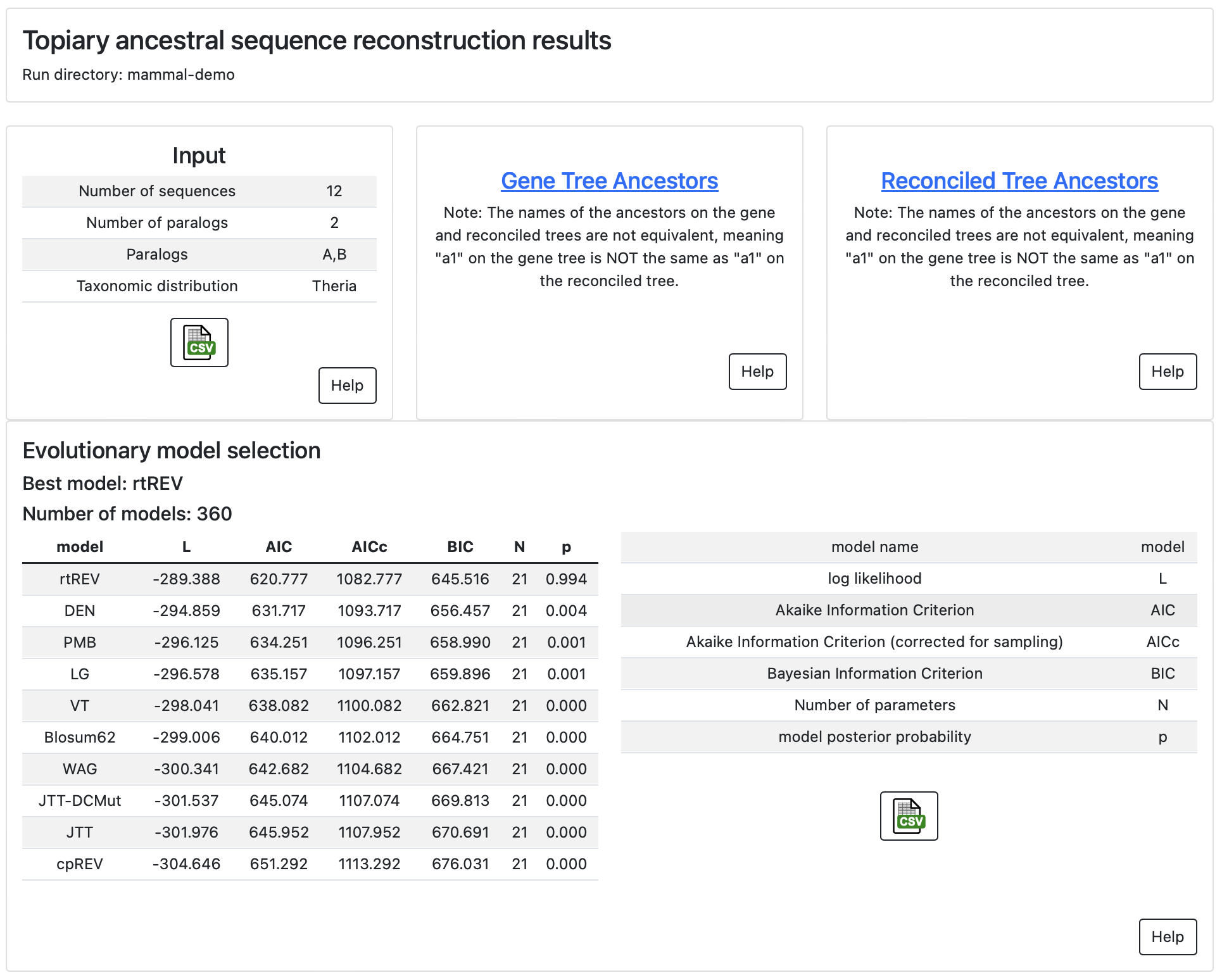
6. Interpret outputs and select ancestors

Danger

Generating ancestors is relatively easy, but experimentally characterizing them can take years; it is worth making sure the ancestors are well reconstructed before ordering genes!

The output from the alignment-to-ancestors and bootstrap-reconcile pipelines will be in the results directory. (This directory is also automatically compressed to results.zip for easy downloading). Open results/index.html in a web browser.

The main page of the report gives information about the input to the inference, a link to the ancestors inferred on the gene tree, a link to ancestors inferred on the and reconciled gene/species tree (if that calculation was done), and information about evolutionary model selection. Each panel has a “Help” button with information about how to interpret the results.

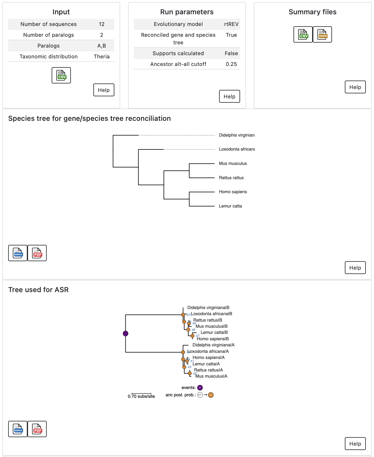
The ancestor pages have information about the input to the calculation, the parameters used for the run, links to summary files, the species tree used (if the gene and species trees were reconciled), and the tree used for the reconstruction. As with the main page, there are “Help” buttons throughout to help you interpret the results.

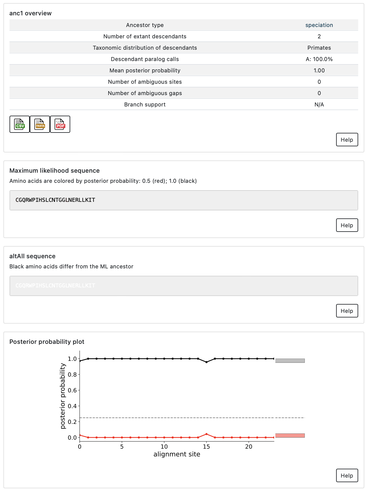
Detailed information is also available for each ancestor. This includes information about ancestor support, sequence, and posterior probability. The “Help” buttons can help interpret the output.

Quality metrics

When you have identified an ancestor you may want to reconstruct, there are two quality metrics to consider deciding to characterize that gene.

The first quality metric is the average posterior probability (PP) for the ML amino acid at all positions in the ancestor. A well reconstructed ancestor would have an average PP of 1.0, meaning the model has high confidence in the sequence at all sites. At the other extreme, a completely ambiguous ancestor would have an average PP of ~1/20 (0.05), meaning each site could have any one of the amino acids. Generally, ancestors in published studies have average PP for the ML reconstructed states > 0.85.

To assess the effect of phylogenetic uncertainty on inferences about the functions of ancestors, we recommend synthesizing two versions of every ancestor. The first is the ML ancestor, as described above. The second is the altAll ancestor. For the altAll ancestor, we replace all ambiguous ML amino acids with the next-most-probable amino acid. If an ancestor has 10 ambiguous sites, the ML and altAll would differ at all 10 of these sites. By functionally characterizing both the ML and altAll versions of an ancestors, we can determine which features are robust to uncertainty in the reconstruction.

A similar sensitivity analysis can be performed if their are ambiguous gaps in the sequence. Topiary does not generate an altAll sequence for gaps; however, ambiguous gaps can be identified by looking in the csv file linked off the ancestor summary page.

The second quality metric is the branch support for a given ancestral node. Posterior probabilities measure our confidence in the ancestral sequence given a particular phylogenetic tree, but they do not measure our confidence in the tree itself. (Put another way, we have the sequence of an ancestral node, but how confident are we that the node existed?) Branch supports measure this confidence.

A branch support measures our confidence that a given group of sequences cluster together, typically on a 0-100 scale. The figure shows branch supports for two possible arrangements of the tree: placing paralog A with B (orange with blue) or paralog B with the fish outgroup (blue with green). In this example we have high support (98/100) for placing paralogs A and B together, with contrasting low support for separating them (2/100). For an ASR study, we need to have high confidence that an ancestral node existed (typically branch support > 85) prior to characterizing the ancestral protein.

Model violation

In addition to checking the posterior probability and branch supports, it is important to make sure the tree topology is reasonable.

The probabilistic models used in ASR are powerful, but do not capture all possible evolutionary events. One common problem is incomplete lineage sorting (ILS), where a gene duplicates but exists as several variants in a population when speciation occurs. Different duplicates are preserved along the descendant lineages, meaning this cannot be classified as a simple duplication or speciation event. ILS is a general problem with all ASR methods and is specifically noted as being outside the scope of GeneRax (the software topiary uses for gene/species tree reconciliation).

Another problem is gene fusion, where different parts of a single gene have different evolutionary histories. The methods used by topiary all assume a single genetic history for each protein sequence. If we force such a model to fit a fused alignment, we will likely end up with a nonsensical evolutionary tree and meaningless ancestral sequences.

A standard signal for both ILS and gene fusion is high discordance between the inferred gene and species trees. This manifests as an unexpectedly high number of duplication and/or transfer events in the reconciled tree. If, for example, you are studying a protein family where you expect two paralogs, but you observe 20 duplication events scattered throughout the tree, there is a good chance that the evolutionary models used for ASR are not appropriate for your protein family.

If topiary detects discordance, it will place a warning in the results for the reconciled tree.

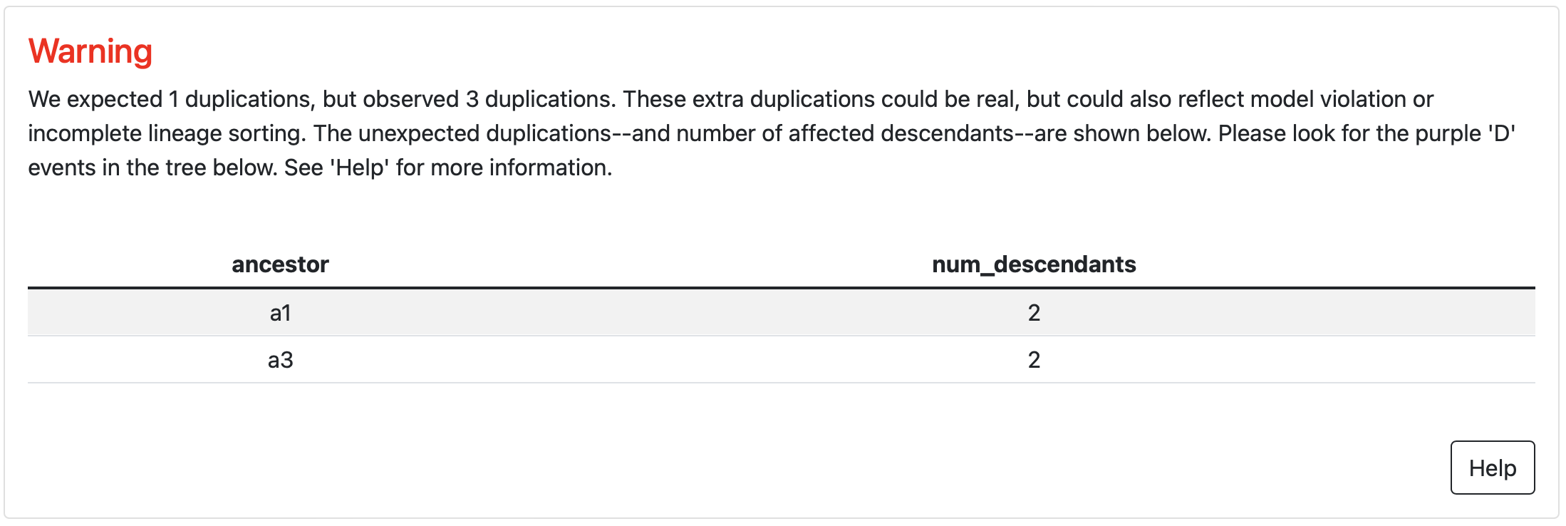
You can find the excess duplications by looking for purple “duplication” nodes in unexpected places on the tree. (In this example, these extra duplications are present in the human and rat.)

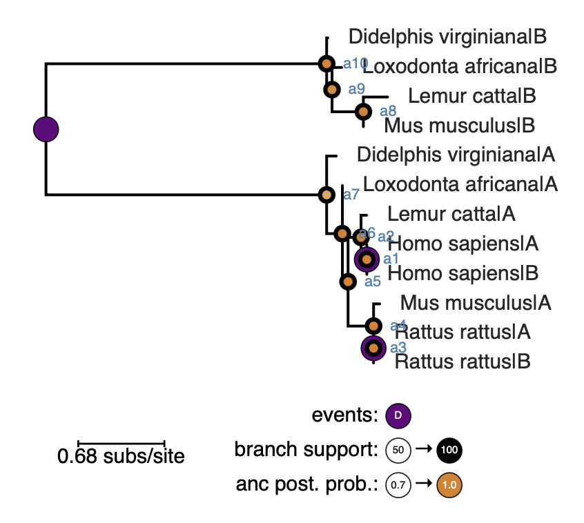
Excess duplications could be observed for benign reasons. The first is lineage-specific duplication, where one or more organisms has more than one copy of a given gene. These will appear as recent duplications near the tips of the tree. The second benign reason would be previously unrecognized gene duplication(s). This will appear as a duplication with taxonomically reasonable descendants. For example, if a gene duplicated in the ancestor of humans, chimps, and gorillas, we would see human/chimp/gorilla on both sides of the duplication event (i.e., six total sequences).

If these conditions are not met, it is likely that model violation is in play.

If your protein has more than one domain, one option would be to try to reconstruct each domain independently. If the discordance disappears, it’s good evidence for a gene fusion event. If the discordance remains, proceed with extreme caution.

Another way forward in the face of discordance is to compare the sequences–and functional characteristics–for any ancestors of interest reconstructed using either the reconciled gene tree and on the gene tree alone. If the results for ancestors reconstructed on the two trees differ dramatically, one cannot infer the ancestral sequence with confidence given standard ASR methods. If the results for the reconstructions on both trees are similar, it suggests whatever features you are trying to reconstruct are robust to uncertainty in the tree topology.